Quantifying and Using Uncertainty in Deep Learning-based UAV Navigation

Quantifying and using uncertainty in Bayesian deep learning systems for robust UAV navigation

Introduction

Autnomous systems, like Unmanned Aerial Vehicles (UAVs) and self-driving cars, increasingly rely on Deep Neural Networks (DNNs) to handle critical functions within their navigation pipelines (perception, planning, and control). While DNNs are powerful, deploying them in safety-critical roles demands that they accurately express their confidence in predictions. This is where Bayesian Deep Learning (BDL) comes in, offering a principled framework to model and capture uncertainty. However, if the Bayesian approach is followed, ideally all the components in the navigation system pipeline (perception, planning, control) should use BDL to enable uncertainty propagation in the pipeline, so that output of the system reflects the uncertainty of the system as a whole . Uncertainty propagation is challeging as it requires BDL components to admit uncertainty information as an input of the DNN to account for the uncertainty coming from previous components.

In this post, we describe how to capture and use uncertainty along a navigation pipeline of BDL components. Moreover, we assess how uncertainty quantificaiton throughout the system impacts the navigation performance of an UAV that must fly autonomously through a set of gates dispoosed in a circle within a simulated environment (AirSim).

The Navigation Task and Architecture Overview

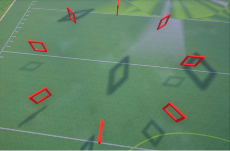
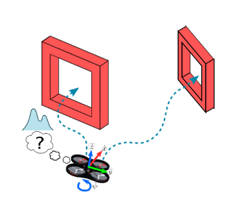
The goal of the autonomous agent (i.e., UAV) is to navigate through a set of gates with unknown locations disposed in a circular track in the AirSim simulator, as presented in Figure 1.

Figure 1: UAV circular track in AirSim.

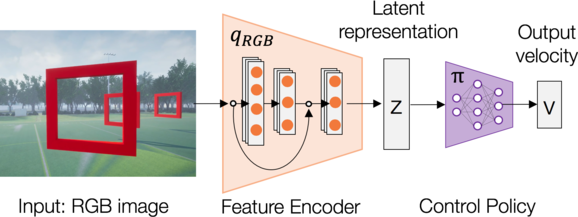
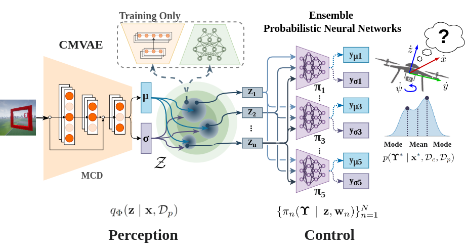
We consider a minimalistic end-to-end deep learning-based navigation architecture to study uncertainty propagation and its use. Therefore, in our experiments, the autonomus navigation architecture consists of two neural network components, one for perception and the other for control, as presented in Figure 2.

Figure 2: UAV autonomous navigation architecture.

To create an instance of the architecture above, we can follow the approach presented in , where the perception component defines an encoder function \(q_{\phi}:\mathcal{X} \rightarrow \mathcal{Z}\) that maps the input image \(\mathbf{x}\) to a rich low dimensional representation \(\mathbf{z} \in \mathbb{R}^{10}\). Next, a control policy \(\pi_{w}: \mathcal{Z} \rightarrow \Upsilon\) maps the compact representation \(z\) to control velocity \(\Upsilon = \{\dot{x}, \dot{y}, \dot{z}, \dot{\psi}\} \in \mathbb{R}^{4}\) commands, corresponding to the desired linear and yaw velocities, respectively in the UAV body frame. This desired velecities are then sent to the UAV low-level controller which is responsible for the UAV motion in the simulator. Figure 3 shows the UAV navigation architecture proposed by Bonatti et al. , where the control policy is implemented using a multilayer perceptron (MLP), and the perception encoder is implemented using the encoder block of a variational autoencoder (VAE).

Figure 3: The input image is encoded into a latent representation of the environment. A control policy acts on the lowerdimensional embedding to output the desired robot velocity commands.

Nevertheless, Bonatti et al. , employ a special type of VAE, a cross-modal VAE (CM-VAE), that allows mixing two data modalities. In the proposed CM-VAE, besides reconstructing the input image, an additional network block is added and trained to predicts the gate’s pose (position and orientation in spherical coordinates) relative to the UAV camera, i.e., the additional network block attached to the VAE performs a (supervised) regression task with the addional data modality (gate pose labels for each image), as presented in Figure 4.

Figure 4: Cross-Modal VAE: Each input image sample is encoded into a single latent space that can be decoded back into images, or transformed into another data modality such as the poses of gates relative to the UAV.

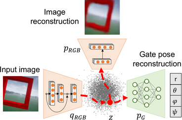
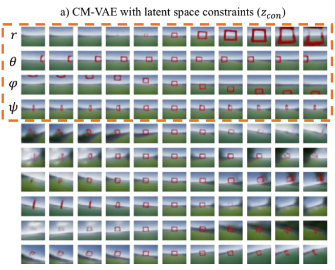
Moreover, the additional network block for predicting the gate poste, is connected in an usual way to the VAE. The regression block only uses the first four variables of the latent vector at the output of the CM-VAE encode. In addition, each of this 4 latent vector variables, is connected to a dedicated regressor for each of the predicted spherical coordinates (radius, polar, azimuth, yaw). This causes a stronger regularization to the latent space during traning since the first 4 variables of the latent space vector will receive an additional flow of error gradients corersponding to pose prediction errors, and therefore, forcing the disentanglement of this 4 latent vector variables, as presented in Figure 5.

Figure 5: CM-VAE disentangled representations: Changing the values from the first four latent vector variables allows us to control the gate attributes in the generated images.

Learning Perception Representations

To build the perception component, we use the Dronet architecture for the CMVAE encoder \(q_{\phi}\). As mentioned before, additional constraints are imposed in the latent space to promote the learning of disentangled representations. For this purpose, the latent vectors \(z\) are treated differently by the decoder \(p_{\theta}\) and the regression networks. The image decoder \(p_{\theta}\) uses the whole latent vector \(z\), while the regression network \(p_{\rho}\) uses only the first four elements \(z_{1:4}\). Each element from \(z_{1:4}\) has a dedicated network to predict a specific gate pose \(\xi\) attribute. Moreover, the CMVAE loss function in Equation \eqref{eq:loss_cmvae_prob} has additional regularization coefficients that penalize the predictions of each network and the closeness to the imposed latent structure.

\[\begin{equation} ({\phi^{*}, \theta^{*}, \rho^{*}}) = \underset{\phi, \theta, \rho}{\arg\min} \text{ } \mathcal{L}_{p}(\mathcal{D}_{p}; \phi, \theta, \rho) \end{equation}\] \[\begin{equation} \mathcal{L}_{p}(\mathcal{D}_{p}; \phi, \theta, \rho) = \mathcal{L}_{p}(\mathbf{x}, \xi; \phi, \theta, \rho) \end{equation}\] \[\begin{equation} \label{eq:loss_cmvae_prob} \mathcal{L}_{p}(\mathcal{D}_{p}; \phi, \theta, \rho) = \frac{\alpha_{p}}{2} {\big\Vert {\mathbf{x} - p_{\theta}(\hat{\mathbf{x}} \mid z)} \big\Vert}^{2} \\ + \frac{\gamma_{p}}{2} {\big\Vert \xi - p_{\rho}(\hat{\xi}\mid z_{1:4}) \big\Vert}^{2}\\ + \beta_{p} \; \mathbb{KL}\big( q_{\phi}(z \mid \mathbf{x}) \; \Vert \; \mathcal{N}(0, \mathbf{I})\big) \end{equation}\]

Learning a Probabilistic Control Policy

Once the perception component is trained, we use only the encoder of the trained CM-VAE to get a rich compact representation (latent vector) of the input image. The downstream control task (control policy $\pi$) uses a MLP network to operate on the latent vectors $z$ at the output of the CMVAE encoder $q_{\phi}$ to predict UAV velocities. To this end, a probabilistic control policy network is added at the output of the perception encoder $q_{\phi}$, forming the UAV navigation stack. The probabilistic control policy network $\pi_{w}(\Upsilon \mid \mathbf{z})$ predicts the mean and the variance for each velocity command given a perception representation $z$ from the encoder $q_{\phi}$, i.e., \(\Upsilon \sim \mathcal{N}\big(\mu_{w}(z), \sigma^{2}_{w}(z)\big)\), where \(\Upsilon_{\mu} = \{\mu_{\dot{x}}, \mu_{\dot{y}}, \mu_{\dot{z}}, \mu_{\dot{\psi}}\}\) and \(\Upsilon_{\sigma^{2}} = \{\sigma^{2}_{\dot{x}}, \sigma^{2}_{\dot{y}}, \sigma^{2}_{\dot{z}}, \sigma^{2}_{\dot{\psi}}\}\). For training the probabilistic control policy, we use imitation learning with a dedicated control dataset $\mathcal{D}_c$, and the heteroscedastic loss function from Equation \eqref{eq:loss_ctrl_policy}.

\[\begin{equation} {w}^{*} = \underset{w}{\arg\min} \text{ } \mathcal{L}_{c}(\mathcal{D}_{c}; w) \end{equation}\] \[\begin{equation} \mathcal{L}_{c}(\mathcal{D}_{c}; w) = \mathcal{L}_{\pi}(\Upsilon, z; w) \end{equation}\] \[\begin{equation} \label{eq:loss_ctrl_policy} \mathcal{L}_{c}(\mathcal{D}_{c}; w) = \frac{1}{2 \hat{\sigma}_{w}^{2}(z)} {\Vert \Upsilon_{i} - \hat{\mu}_{w}(z) \Vert}^{2} + \frac{1}{2} \log \hat{\sigma}_{w}^{2}(z) \end{equation}\]

Following the work by , during training, we freeze the weights fromt the perception encoder $q_{\phi}$ to update only the weights $w$ from the control policy network, as presented in the control component from Figure 7.

Autonomous Navigation Overview

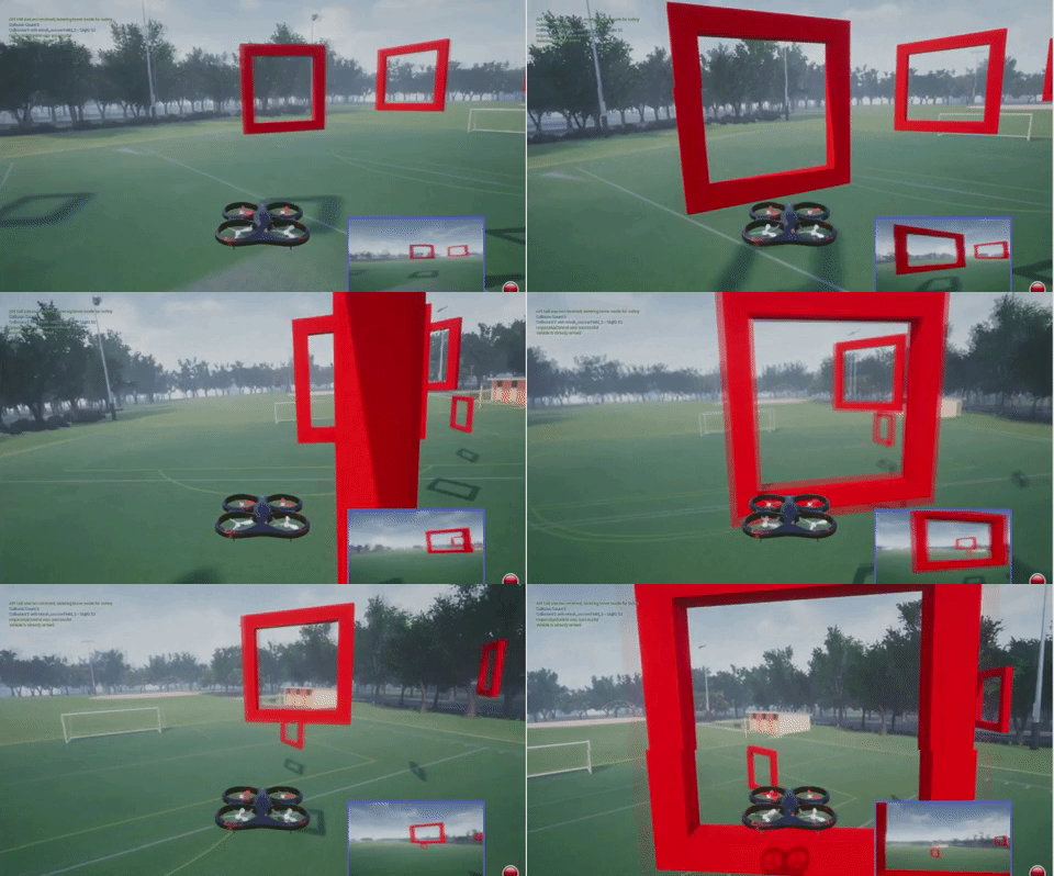
After training the components of the minimalistic navigation architecture, we obtain autonomous navigation flight that drives the UAV through the red gates as shown in Figure 6.

Figure 6: UAV autonomous navigation in AirSim simulator.

Quantifying Uncertainty in the DNN-based Navigation System

Uncertainty From Perception Representations

Although the CMVAE encoder \(q_{\phi}\) employs Bayesian inference to obtain latent vectors \(\mathbf{z}\), CMVAE does not capture epistemic uncertainty since the encoder lacks a distribution over parameters $\phi$. To capture uncertainty in the perception encoder, we follow prior work from that attempts to capture epistemic uncertainty in VAEs. We adapt the CMVAE to capture the posterior \(q_{\Phi}(\mathbf{z} \mid \mathbf{x}, \mathcal{D}_p)\) as shown in Equation \eqref{eq:postEncoder}.

\[\begin{equation} \label{eq:postEncoder} q_{\Phi}(\mathbf{z} \mid \mathbf{x}, \mathcal{D}_{p}) = \int{q(\mathbf{z} \mid \mathbf{x}, \phi) \; p(\Phi \mid \mathcal{D}_{p}) \; d\phi} \end{equation}\]

To approximate Equation \eqref{eq:postEncoder} we take a set \({\Phi = \{\phi_{m}\}^{M}_{m}}\) of encoder parameter samples \(\phi_{m} \sim p(\Phi \mid \mathcal{D}_{p})\), to obtain a set of latent samples \(\{z_{m}\}^{M}_{m=1}\) from the output of the encoder \(q_{\Phi}(\mathbf{z} \mid \mathbf{x}, \mathcal{D}_{p})\). In practice, we modify the CMVAE by adding a dropout layer in the encoder. Then, we use Monte Carlo Dropout (MCD) to approximate the posterior on the encoder weights \(p(\Phi \mid \mathcal{D}_{p})\), as shown for the perception component in Figure 7. Finally, for a given input image \(\mathbf{x}\), we perform \(M\) stochastic forward passes (with dropout turned on) to compute a set of \(M\) latent vector samples \(\mathbf{z}\) at runtime.

Figure 7: Uncertainty-aware UAV navigation architecture.

Handling Input Uncertainty In The Control Policy

In BDL, downstream uncertainty propagation assumes that a neural network component is able to handle or admit uncertainty at the input. In our case, this implies that the neural network for control is able to handle the uncertainty coming from the perception component. To do that we consider using the BNN with LV inputs (BNN+LV) approach to propagate the uncertainty from perception to control in a principled way. To capture the overall system uncertainty at the output of the controller, we compute the posterior predictive distribution for target variable \(\Upsilon^{*}\) associated with a new input image $\mathbf{x}^{*}$, as shown in Equation \eqref{eq:postPredDist} and Equation \eqref{eq:post_pred_dist_whole_system}:

\[\begin{equation} \label{eq:postPredDist} p(\Upsilon^{*} \mid \mathbf{x}^{*}, \mathcal{D}_{c}, \mathcal{D}_{p}) = \iint{\pi(\Upsilon} \mid \mathbf{z}, \mathbf{w}) \;p(\mathbf{w} \mid \mathcal{D}_{c}) \;q_{\Phi}(\mathbf{z} \mid \mathbf{x}^{*}, \mathcal{D}_{p}) \;dz \;dw \end{equation}\] \[\begin{multline} \label{eq:post_pred_dist_whole_system} p(\Upsilon^{*} \mid \mathbf{x}^{*}, \mathcal{D}_{c},\mathcal{D}_{p}) = \\\int \int \int \underbrace{\pi(\Upsilon^{*} \mid \mathbf{z}, \mathbf{w})}_\textit{control policy} \; p(\mathbf{w} \mid \mathcal{D}_{c}) \underbrace{q(\mathbf{z} \mid \mathbf{x}^{*}, \Phi)}_{\textit{perception encoder}} p(\Phi \mid \mathcal{D}_{p})\; d\phi \; dz \; dw \end{multline}\]

The integrals from the equations above are intractable, and we rely on approximations to obtain an estimation of the predictive distribution. The posterior \(p(\mathbf{w} \mid \mathcal{D}_{c})\) is difficult to evaluate. Thus, we can approximate the inner integral using an ensemble of neural networks . As presented in Figure 7, in practice, we train an ensemble of $N$ probabilistic control policies \({\pi}_{w_{n}}(\Upsilon \mid \mathbf{z}, w_{n})\), with weights \(\{w_{n}\}^{N}_{n=1} \sim p(\mathbf{w} \mid \mathcal{D}_{c})\), and where each control policy \({\pi}_{w_{n}}\) in the ensemble predicts the mean $\mu_{w_{n}}(\mathbf{z})$ and variance \(\sigma^{2}_{w_{n}}(\mathbf{z})\) for each velocity command, i.e., \(\Upsilon \sim \mathcal{N}\big(\mu_{w_{n}}(\mathbf{z}), \sigma^{2}_{w_{n}}(\mathbf{z})\big)\).

The inner integral is approximated by taking a set of samples from the perception component latent space. Latent representation samples are drawn using the encoder mean and variance \(\mathbf{z} \sim \mathcal{N}(\mu_{\phi},\sigma^{2}_{\phi})\). For brevity, we directly use the samples obtained in the perception component \(\{z_{m}\}^{M}_{m} \sim q_{\Phi}(\mathbf{z} \mid \mathbf{x}, \mathcal{D}_{p})\) to take into account the epistemic uncertainty from the previous stage. Finally, the predictions we get from passing each latent vector $\mathbf{z}$ through each ensemble member are used to estimate the posterior predictive distribution in Equation \eqref{eq:postPredDist}. The predictive distribution \(p(\Upsilon^{*} \mid \mathbf{x}^{*}, \mathcal{D}_{c},\mathcal{D}_{p})\) from Equation \eqref{eq:post_pred_dist_whole_system}, takes into account the uncertainty from both system components.

From the control policy perspective, using multiple latent samples $\mathbf{z}$ can be seen as taking a better “picture” of the latent space (perception representation) to gather more information about the environment. Interestingly, we can also make a connection between our sampling approach and the works that aim at sampling the input space by performing translations and augmentations on input images to improve prediction robustness.

Finally, to control the UAV, we use the deep ensemble expected value of the predicted velocities, as suggested in the literature . This means that we use, \(\mathbf{\hat{y}}_{\mu} = \mathbb{E}([\mu_{\dot{x}}, \mu_{\dot{y}}, \mu_{\dot{z}}, \mu_{\dot{\psi}}])\). These predicted velocities represent the desired or reference velocities that are passed to AirSim’s low-level control through its API.

Navigation Performance Evaluation

The goal of the UAV is to navigate through a set of gates with unknown locations, forming a circular track. In AirSim, a track is entirely defined by a set of gates, their poses in the space, and the agent navigation direction. For perception-based navigation, the complexity of a track resides in the “gate-visibility” difficulty , i.e., how well the UAV camera Field-of-View (FoV) captures the target gate.

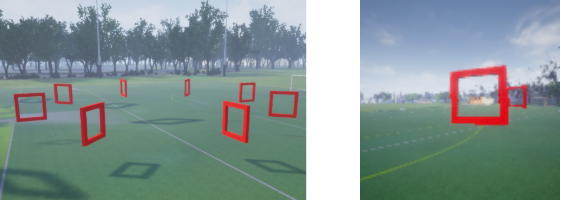
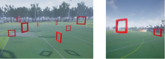
We evaluate the navigation system using a circular track with eight equally spaced gates positioned initially at a radius of 8 m and constant height, as shown in Figure 8. A natural way to increase track complexity is by adding a random displacement to the position of each gate in the track, i.e., introducing operational domain shift (a factor that influences model predictive uncertainty). A track without random displacement in the gates has a circular fashion. Gate position randomness alters the shape of the track, affecting the gate visibility, as presented in Figure 9, and therefore, the generation of shifted images is more likely to happen, e.g., gates are “not visible, partially visible, or multiple gates” can be captured in the UAV FoV.

Figure 8: UAV navigation circular track without noise. Birds-eye view (left), and the UAV view perspective (right).

Figure 8: UAV navigation circular track with noise. Birds-eye view (left), and the UAV view perspective (right).

To assess the system performance and robustness to perturbations in the environment, we generate new tracks adding an offset to each gate radius and height with random noise. We specify the Gate Radius Noise (GRN) and the Gate Height Noise (GHN) with two levels of track noise, as follows:

\[\begin{align*} \text{Noise level 1} \begin{cases} GRN \sim \mathcal{U}[-1.0, 1.0)\\ GHN \sim \mathcal{U}[0, 2.0) \end{cases} & \;\;\;\;\; \text{Noise level 2} \begin{cases} GRN \sim \mathcal{U}[-1.5, 1.5)\\ GHN \sim \mathcal{U}[0, 3.0) \end{cases} \end{align*}\]

In this regard, with this experimental setup we seek to answer the following research question:

RQ-1: Can we improve the UAV performance and robustness to perturbations of the environment by using an uncertianty-aware DL-based navigation architecture?

Navigation Models Setup

Navigation Models Trainind Datasets. We use two independent datasets for each component in the navigation pipeline. The perception CMVAE uses a dataset ($\mathcal{D}_p$) of 300k images where a gate is visible and gate-pose annotations are available. The control component uses a dataset ($\mathcal{D}_c$) of 17k images with UAV velocity annotations. $\mathcal{D}_c$ is collected by flying the UAV in a circular track with gates, using traditional methods for trajectory planning and control. The perception dataset is divided into 80\% for training and the remaining 20\% for validation and testing. The control dataset uses a split of 90\% for training and the remaining for validation and testing. In both cases, the image size is 64x64 pixels.

Navigation Models Baselines. Ideally, we would expect the UAV to have a more robust and stable navigation performance with a full uncertainty-aware navigation architecture and by using the expected value of the predicted velocities , at the output of the system or the control component. To see if this premise holds, we compare the navigation performance from different UAV uncertainty-aware navigation architectures. The navigation models are listed below in Table 1, showing the uncertainty-aware navigation architectures used in our experiments, and detailing the type of perception component, the number of latent representation samples (LRS), the type of control policy, and the number of control prediction samples (CPS) at the output of the system, as presented below:

Navigation Model	Perception Encoder	LRS	Control Policy	CPS

Table 1: UAV navigation models.

In Table 1, models $\mathcal{M}_1$ to $\mathcal{M}_3$ partially capture uncertainty in the pipeline since they use a deterministic perception component (CMVAE). For the control component, $\mathcal{M}_1$ and $\mathcal{M}_2$ take 32 and 1 LRS, respectively, and use the samples later with an ensemble of 5 probabilistic control policies capturing epistemic and aleatoric uncertainty. $\mathcal{M}_3$ uses 32 LRS, and the control component is completely deterministic. Finally, $\mathcal{M}_4$ represents our Bayesian navigation pipeline where the perception component captures epistemic uncertainty using MCD with 32 forward passes for each input to get 32 latent representation predictions. To ease the computation, perception predictions are directly used as latent variable samples in downstream control. The control component uses an ensemble of 5 probabilistic control policies, obtaining 160 control prediction samples.

Results

Table 2, shows the UAV navigation models performance. Moreover, the videos below we observe a qualitative performance comparison of each model in the UAV navigation task.

Navigation Model	Gates Passed @ Track Noise Level 1	Gates Passed @ Track Noise Level 2

Table 2: UAV navigation models performance.

UAV navigation model M1

UAV navigation model M2

UAV navigation model M3

UAV navigation model M4

Based on the results of the experiments, we can answer RQ-1 saying that the uncertainty-aware DL-based navigation architecture marginally improves the UAV performance and robustness to perturbations of the environment. But the surprising point here is that the performance from the full Bayesian navigation architecture $\mathcal{M}_4$ is slightly better than partial uncertianty-aware archictecture $\mathcal{M}_2$. This situation allow us to question the benefit of the full Bayesian navigation architecture, and more precisely, the tradeoff between performance & robustness benefit vs. the required computational resources, since the simple partial uncertainty-aware $\mathcal{M}_2$ provides similar performance.

Naturally, based on these observations, our next question is:

RQ-2: What is the reason for this behavior and performance in the full uncertainty-aware (Bayesian) architecture $\mathcal{M}_4$ compared to other partial uncertainty-aware navigation architectures?

Leveraging System Uncertainty for Better Navigation Performance

Understanding the System Components’ Predictive Uncertainty

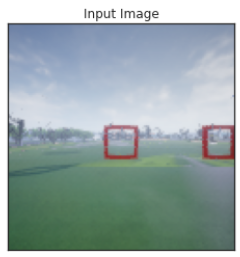
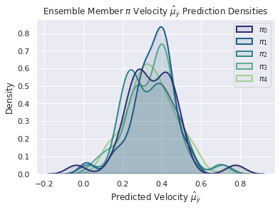
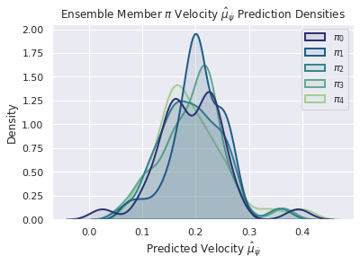
To try to understand what is going on during the UAV autonomous mission/task execution, lets probe the predictions of each component of the fully Bayesian navigation architecture, when facing one of the situations that arises when adding noise to the tracks as shown in Figure 8. In particular, consider the double-gate case from Figure 9 and its generated predictions in Figure 10 below:

Figure 9: Double gate situation in the UAV field-of-view caused by noisy circular tracks (left). UAV field-of-view and the corresponding input image for the DNN when double-gate situation (right).

Figure 10: Predicted (mean $\hat{\mu})$ lateral velocity $\dot{y}$ and yaw angular velocity $\dot{\psi}$, for each control component ensemble member $\pi$.

This controlled experiment reveals that the introduced ambiguity (two gates) in the input image for the UAV DNN-based navigation architecture, is also reflected in the predicted control actions. The predicted control commands that will move the UAV towards one of the two gates, i.e., $\hat{\dot{y}}$ (lateral vel. left or right) and $\hat{\dot{\psi}}$ (yaw rotation cw and ccw), present multimodal distributions fo reach ensemble member in the control component. This situation suggest the posibility of two likely values for the control command, which is a clear indication of the uncertainty in the control command.

Conclusion

TBD

For more in depth info about this topic, please check the papers .