Notes on Simple Approximate Inference in Bayesian Neural Networks
Deep Neural Networks Uncertainty
Disclaimer: The notes from this post were taken from the works listed in the References section.
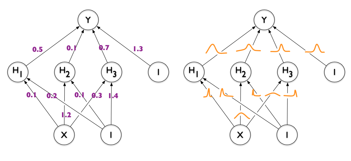 Figure 1: Deterministic Neural Network vs Bayesian Neural Network
The main benefit of using a Bayesian framework is that allows to propagate uncertainty to improve prediction and model reasoning. In this sense, is important that each component of a system computes an accurate estimate of uncertainty to later reflect the true uncertain in the system.
Metrics must capture the quantitative performance of the uncertainty the model is trying to measure.
Typical metrics should include uncertainty calibration plots and precision recall statistics of regression and classification algorithms.
Task-specific metrics include inspecting test-log-predictive-probabilities a measure of how “surprised” the system output is on a test-set of known outcomes
It is most important to accurately quantify the uncertainty of intermediate representations, such as those from perception and scene prediction components.
The most important aspect is to correctly propagate uncertainty to the following layers so that we can make informed decisions. The final control output will be a hard decision. Therefore uncertainty metrics should focus on intermediate components and tasks such as perception, sensor fusion and scene prediction
Notes taken from [1]
Bayesian Uncertainty Estimation
- Uncertainty is Used to track the dependability of the model.
- In classification problems, softmax probabilities are not enough to indicate whether the model is confident in its prediction.
- A standard model would pass a point estimate through the softmax layer rather than the whole predictive distribution. This lead to high probabilities or high confidence on points far from data.
- An example of Out-of-Distribution sample: In self-driving, if the training set of a model consisted of only images from highways and the model was then given an image of a dirt track, the model would return a steering angle but we would ideally require the model to have high uncertainty
- Noisy data $\rightarrow$ Aleatoric uncertainty
- Model parameters uncertainty/variability $\rightarrow$ Epistemic uncertainty
- Means to estimate epistemic uncertainty is to perform Bayesian Inference.
Notes taken from [2]
Epistemic Uncertainty Estimation with Bayesian Inference
The aim is to use the posterior distribution $p(\theta \mid D)$ which is obtained from the data likelihood and the prior $p(\theta)$ by applying Bayes theorem. The uncertainty in the model parameters is then marginalized out to obtain the posterior distribution:
\[p(y^{*} \mid x^{*}, D) = \int p(y^{*} \mid x^{*}, \theta) p(\theta \mid D) d\theta\]The general intractable integral from above is approximated using $M$ Monte Carlo samples $\theta^{i}$, ideally from the posterior. However, in practice is virtually impossible for DNNs to obtain samples from the true posterior $p(\theta \mid D)$. This requires approximation methods $q(\theta) \approx p(\theta \mid D)$ to be used [4].
\[p(\theta \mid D) = \frac{p(D \mid \theta) p(\theta)}{p(D)}\]The probability distribution of interest is the distribution $p$ of the parameters $\theta$ after the data $D$ is seen. $p(D \mid \theta)$ is the likelihood of the occurrence of data $D$ given a model with parameters $\theta$, $p(\theta)$ the prior, and $p(D)$ the data distribution. Incorporating a prior belief in investigating a posterior state is a central characteristic of Bayesian reasoning. This prior is hence often referred to as domain knowledge [5].
Learning for the BNN, amounts to computing the posterior distribution over the weights, $p(w \mid D)$ through Bayes Rule. Because of the non-linearity introduced by the Neural Network architecture, the computation of the posterior cannot be done analytically. Hence various approximation methods have been studied to perform inference with BNNs in practice [3], these methods are listed below:
Markov Chain Monte Carlo Methods
Hamiltonian Monte Carlo (HMC):
Proceeds by defining a Markov chain whose invariant distribution is $p(w \mid D)$ or $p(\theta \mid D)$. Relies on Hamiltonian dynamics to speed up the exploration of the space. HMC does not make any assumptions on the form of the posterior distribution, and is asymptotically correct. The result of HMC is a set of samples $w_{i}$ or $\theta_{i}$ that approximate $p(w \mid D)$ or $p(\theta \mid D)$ [3].
Variation Inference Methods
Proceeds by finding a Gaussian approximate distribution $q(w) \approx p(w \mid D)$ in a trade-off between approximation accuracy and scalability. The core idea is that $q(w)$ depends on some hyper-parameters that are then iteratively optimized by minimizing a divergence measure between $q(w)$ and $p(w \mid D)$. Samples can then be efficiently extracted from $q(w)$ [3].
Monte Carlo Dropout (MCD):
A particularly simple and scalable variant. The method entails using dropout also at test time, which can be interpreted as performing Variational Inference (VI) with a Bernoulli variational distribution. The approximate predictive posterior is obtained by performing $M$ stochastic forward passes on the same input [4].
\[p(y^{*} \mid x^{*}, D):= \frac{1}{M} \sum_{i=1}^{M}p(y^{*} \mid x^{*}, \theta^{(i)}), \space \space \theta^{(i)} \sim p(\theta \mid D)\]
Ensembling (considered also non-bayesian)
The parametric model $p(y \mid x, \theta)$ of the conditional distribution was created using a DNN $f_{\theta}$, and learned multiple point estimates ${\hat{\theta}^{(m)}}_{m=1}^{M}$, by repeatedly minimizing the MLE objective $log\space p(Y \mid X, \theta)$ with random initialization. They then averaged over the corresponding parametric models to obtain the predictive distribution:
\[p(y^{*} \mid x^{*}, D):= \frac{1}{M} \sum_{m=1}^{M}p(y^{*} \mid x^{*}, \theta^{(m)})\]This approach is considered as a non-Bayesian alternative to predictive uncertainty estimation. However, since ${\hat{\theta}^{(m)}}_{m=1}^{M}$, always can be seen as samples from some distribution $\hat{q}(\theta)$, we note that the previous equation is virtually identical to the equation described in MCD section. Ensembling can also be viewed as approximate Bayesian inference, where the level of approximation is determined by how well the implicit sampling distribution $\hat{q}(\theta)$ approximates the posterior $p(\theta \mid D)$ [4].
Uncertainty Metrics
It has been shown that a networks that uses dropout is an approximation to a Gaussian Process, where $\mathbf{f}$ is the space of functions, $\mathbf{X}$ is the training data and $\mathbf{Y}$ is the training outputs. The expectation of $\mathbf{y^{*}}$ is called the predictive mean of the model and the variance is the predictive uncertainty [2].
\[p(\mathbf{y^{*}} \mid \mathbf{x^{*}}, \mathbf{X}, \mathbf{Y}) = \int p(\mathbf{y^{*}} \mid \mathbf{f^{*}}) \space p(\mathbf{f^{*}} \mid \mathbf{x^{*}}, \mathbf{X}, \mathbf{Y}) \mathrm{d}\mathbf{f^{*}}\]Regression
For a regression network, the following equations are used to obtain an approximation of the predictive mean and variance of a Gaussian Process. Note that a network that uses dropout approximates a Gaussian Process [2].
\[\mathrm{E(y^{*})} \approx \frac{1}{T} \sum_{t=1}^{T}\hat{\mathrm{y}}^{*}_{t} (\mathrm{x^{*}})\] \[\mathrm{Var(y^{*})} \approx \tau^{-1} \mathbf{I}_\mathrm{D} + \frac{1}{T} \sum_{t=1}^{T}\hat{\mathrm{y}}^{*}_{t}(\mathrm{x^{*}})^T \space \hat{\mathrm{y}}^{*}_{t} (\mathrm{x^{*}}) - \mathrm{E(y^{*})}^T \mathrm{E(y^{*})}\]The set ${\mathrm{\hat{y}}_{t} (\mathrm{x^{*}})}$ of size $T$ is the results from $T$ stochastic forward passes through the network. It is important that the non-determinism from dropout is retained at prediction time to ensure different units will be dropped per pass through. Relating back to the Gaussian process, these are empirical samples from the approximate predictive distribution seen in Equation (5). $\tau$ relates to the precision of the Gaussian process model, and is used in the calculation of the predictive variance [2]. $\tau$ can be calculated as follows:
\[\tau = \frac{l^{2} p}{2 N \lambda}\]where $l$ is a user-defined length scale, $p$ is the probability of units not being dropped, $N$ is the number of training samples and $\lambda$ is multiplier used in the L2 regularization of the network.
Classification
Softmax probabilities are a poor indicator of model prediction confidence, as they are the result of a single deterministic pass of a point estimate through the network. This situation can lead to high confidence on points far from the training data[2] that potentially wrong. The approaches to quantify classification uncertainty are:
- Variation Ratios
- Predictive Entropy
- Mutual Information
References
Concrete Problems for Autonomous Vehicle Safety: Advantages of Bayesian Deep Learning. R McAllister, Y. Gal, A. Kendall, et al. IJCAI 2017
Evaluating Uncertainty Quantification in End-to-End Autonomous Driving Control. R Michelmore, M Kwiatkowska, Y Gal. 16/11/2018
Uncertainty Quantification with Statistical Guaranteees in End-to-End Autonomous Driving Control. R Michelmore, M Wicker, L Laurenti, L Cardelli, Y Gal, M Kwiatkowska. 21/09/2019
Evaluating Scalable Bayesian Deep Learning Methods for Robust Computer Vision. F K Gustafsson, M Danelljan, et al. 04/06/2019
Probabilistic Deep Learning: Bayes by Backprop. Felix Laumann.